Learning how to add a check mark in Excel is a valuable ability to have, especially when you want to make your spreadsheets look more professional, organized, and clean-cut. Accessing check marks in Excel is not as straightforward as it could be, but we are here to help.

Fortunately, there are various methods for creating tick marks in Excel. You can use keyboard shortcuts or, if you like, manually go to a symbols dialogue box to add an Excel check mark in this manner. 

In this post, we’ll teach you how to insert a checkmark in Excel, as well as why and how to use it.

Excel’s Check Mark Symbol

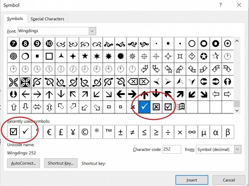
The check symbol (✓) is a unique character seen in spreadsheets as well as other digital documents, such as documents created using Word. If you’re working with Microsoft Excel, you can add this character by utilizing the Symbol dialogue box, which contains the majority of the standard Excel symbols.

To get the Symbol dialogue box in Excel, go to the “Insert” tab on the Ribbon, then select “Symbol.”

Select “Symbol” within the Font drop-down list in the Symbol dialogue box, then go down in the “Symbols” list until you locate the tick symbol. Once you’ve located it, click “Insert” to place a checkmark in the cell.

How to Add a Checkmark In Excel through a Keyboard Shortcut

How to type a check mark? If you’re going to put check marks into your spreadsheet in Excel on a frequent basis, it might be faster to set up a check mark on keyboard shortcut instead of accessing the Symbol dialogue box each time. To insert check mark in Excel via keyboard shortcut, go to the “File” menu and select “Options.”

Click “Customize Ribbon” in the left panel of the “Excel Options” dialogue box. Click the “Main Tabs” check box in the “Customize the Ribbon” section to pick it, then click “OK.”

The Ribbon will now have a “Developer” tab. Select the “Developer” tab, then select “Macros” from the “Code” group. This brings up the “Macros” dialogue box.

Select “All Open Workbooks” from the “Macros in” drop-down list, then click “Create.” The Microsoft Visual Basic for Applications editor will be launched.

Enter the following code in the editor:

Sub ActiveCell.Value = ChrW(&H2713) InsertCheckMark(✓)Finish Sub

This code adds a checkmark to the active cell. To make the keyboard shortcut, go to “Tools,” then “Macro,” and finally, “Macros.” Select “InsertCheckMark” from the list in the “Macros” dialogue box, then click “Options.”

Click on the “Shortcut key” text box in the “Assign Macro” dialogue box, then write the keyboard action you would like to use. You could, for example, use the “Alt+C” shortcut. When you’ve finished typing the shortcut, click “OK,” then “Close.”

To enter a checkmark into a cell now, simply pick the cell and use the keyboard shortcut for checkmark. The checkmark is going to be placed inside the cell.

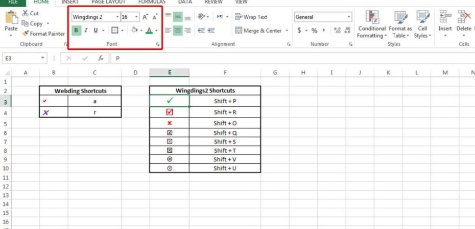
How to Put a Checkmark In Excel using the Wingdings Font

How to insert check box in Excel? The Wingdings typeface can also be used to insert a tick mark into an Excel cell. You can insert a tick mark symbol into a cell with this font. To do so, first, select the cell where you wish to place the checkmark.

On the Ribbon, select the “Home” tab, then the “Font” drop-down list under the “Font” group. Choose “Wingdings” from the font list.

After you’ve decided on the Wingdings typeface, enter the letter “a” into the cell. A wingdings checkmark will be added to the cell as a result of this.

How to Add a Checkmark In Excel to a Header or Footer

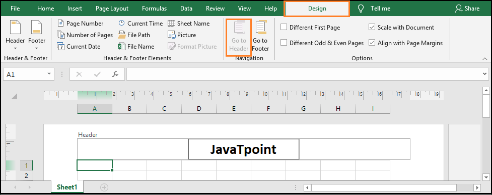
If you wish to enter a checkmark into an Excel spreadsheet’s header or footer, use the “Header & Footer Elements” button. To do so, navigate to the “Insert” section on the Ribbon and then to “Header & Footer.”

Click the “Header & Footer Elements” button in the “Header & Footer” section. This will bring up a selection of headers as well as footer items that you may add to the header or footer.

From the menu, choose “Field.” This will add a field to the header or footer of your page. Select “Symbol” from the “Category” drop-down list in the “Field Codes” dialogue box.

Select the tick mark symbol from the “Symbols” list, then click “Insert.” The checkmark will be added to the header or footer of your document.

How to Add a Checkmark In Excel through an Equation

How to add a check box in Excel? An equation can also be used for putting a checkmark into a cell. 

1. First, select the cell where you wish to place the checkmark.
2. Select the “Insert” tab on the Ribbon, followed by “Equation.” This will put a formula into the cell.
3. Click the “Symbols” button in the “Equation Tools” Ribbon. The “Symbols” dialogue box will appear.
4. Select “Normal Text” from the “Subset” drop-down list in the “Symbols” dialogue box.
5. Scroll down until you see the tick mark symbol in the “Symbols” list, then click “Insert.” This will place a checkmark in the cell.

How to Add a Checkmark in Excel through the UNICHAR Function

The UNICHAR function is a formula that converts numeric codes into equivalent characters and is the simplest way to put a check mark symbol in Excel. Check marks in Excel can be represented by four UNICHAR codes: 9745, 9989, 10003, and 10004. Here’s where to begin.

1. Choose a cell in which to place your tick mark.
2. Enter “=UNICHAR” accompanied by one of the previously specified codes enclosed in brackets. If you want to utilize the 10003 code, for example, your submission should look like this: =UNICHAR(10003)
3. Pressing the “Enter” key should display the tick mark.

How to Add a Checkmark through an ASCII Code

An ASCII code can also be used to enter a checkmark in a cell. ASCII check mark codes are characters in a digital document that are represented by codes. The ASCII code for the tick mark symbol is ✓

1. To place a checkmark in a cell through an ASCII code, pick the cell into which the checkmark is to be inserted.
2. On the Ribbon, select the “Insert” option, then “Symbol.” In the “Symbol” dialogue box, choose “More Symbols.”
3. Select “Unicode (Hex)” from the “From” drop-down list in the “Symbols” dialogue box.
4. Enter ✓ in the “Character Code” text box, then click “Insert.” This will place a checkmark in the cell.

How to Add a Checkmark through a Character Code

You can also put a tick mark into a cell if you have the character code for the checkmark symbol. The tick mark symbol has the character code ✓

1. First, to place a checkmark in a cell through a character code, pick the cell into which the checkmark is to be inserted.
2. On the Ribbon, select the “Insert” option, then “Symbol.” In the “Symbol” dialogue box, choose “More Symbols.”
3. Select “Unicode (Hex)” from the “From” drop-down list in the “Symbols” dialogue box.
4. Enter ✓ in the “Character Code” text box, then click “Insert.” This will place a checkmark in the cell.

How to Add a Checkmark through a Character Map

The Character Map tool can also be used for placing a checkmark in a cell. You can use this tool for adding special characters to an Excel spreadsheet. Click the “Start” button, then put “character map” into the search area to open the Character Map tool. To access the tool, select “Character Map” from the results.

Select “Wingdings” from the “Font” drop-down list in the “Character Map” dialogue box.

Scroll down until you see the tick mark symbol in the “Characters” section, then click “Select.” This will place a checkmark in the cell.

How to Add Check Marks In Excel by Converting True False to Checkbox

If you are using a column in the Excel sheet labeled “TRUE” or “FALSE,” you may use this method to turn it into a checkbox.

1. Make a new column adjacent to the one that contains the “TRUE” or “FALSE” values.
2. In the first cell of the new column, enter the following formula: =IF(A1=TRUE, “,”
3. In the formula, replace “A1” with the cell reference of the first cell in the column containing the “TRUE” or “FALSE” values.
4. Drag the formula to the new column’s bottom.
5. Right-click the “Format” button, then select the “Font” option.
6. Choose “Wingdings” as the font type in the “Font Style” section.
7. To go back to the worksheet, press the “OK” button.
8. Drag the formula to the bottom of the freshly created column to replace cells with tick boxes.

How to Switch the Color of the Checkmark

To alter the color of the checkmark, pick the cell and then click the “Home” tab on the Ribbon. Click the “Font Color” drop-down list in the “Font” group and choose the color you wish to use.

How to Get Rid of a Checkmark

To delete the tick mark from a cell, select it and then use the “Delete” key on the keyboard. This removes the check mark from the cell.

How to Remove All Tick Marks in an Excel Workbook in One Go?

You can use the Find and Replace feature to delete all check marks in a Microsoft Excel workbook simultaneously. Here’s how to go about it:

1. 1. Choose every single cell in the workbook by pressing Ctrl+A.
2. 2. In the Ribbon, choose the Home tab.
3. 3. Select “Replace” from the Find & Select drop-down list.
4. 4. Insert the character code for the checkmark in the “Find what” area.
5. 5. Keep the “Replace with” box empty.
6. 6. Press the “Replace All” option.
7. 7. Hit “OK” to check that all tick marks have been removed.
8. 8. Click OK to exit the Find and Replace dialogue box.

This will clear out all of the tick marks in your Excel workbook.

Where Should a Checkmark be Used in Excel?

When preparing spreadsheets at work, including tick marks in the spreadsheet may be helpful. Here are some examples of when you could utilize the symbol in a single cell:

To organize the contents of an Excel spreadsheet

A tick mark may fulfill the same function as a bullet point, which can assist in arranging the material of your spreadsheet. The tick mark can be used to represent the following item in a series as well as the beginning of a new row of information. When you have a standard collection of symbols in the text, it may be simpler for readers to review the statistics you computed or the conclusions you’ve formed. For example, you could include a tick mark beside their names on the Excel sheet to reflect the total number of clients that paid invoices.

To add an aesthetic appeal to an Excel report

Check marks can also be used to enhance the visual appeal of reports created in Excel. You can use a tick mark instead of words to signify that you’ve successfully completed an item. The improved visual appeal also allows you to keep your report brief, making it easier to relay essential data to the people reading your document. For example, if you are in charge of a team, you could use an Excel sheet to describe the goals for a future project. The tick marks might help specialists grasp your expectations and discern critical aspects.

To show the progress of a work assignment

Check marks in a spreadsheet program can also help create a list of items to complete for what you have to do on a given workday. The symbols can show you which assignments you’ve completed, which might help you track your productivity. As you continue, mark the task on the Excel sheet with a tick mark. The ones that are without a sign indicate that you intend to accomplish them. If you operate with a team, tick marks on to-do lists may assist you and your colleagues in evaluating group productivity.

Tips for Adding a Checkmark in Excel

Explore the following recommendations for further information on utilizing unique symbols in spreadsheet software:

Altering the size and color

Consider adjusting the size and color of the tick mark once you’ve added it to a cell. You can increase the prominence of the symbol on the page to verify that it is appropriately aligned with the balance of your text. Altering the setting of the tick mark within the cell is another possibility. You can move the sign to the right, center, or left using the “Alignment” box.

For example, to indicate completed items on a checklist, you may change the color of the tick mark to green. Choose a design that adds to the overall aesthetic of the report. You may also ensure that readers can clearly see the tick marks as they scan the spreadsheet’s content.

Go through the selection of checkmarks.

Excel also allows you to add many types of tick marks to your document. Each of them has a unique character code. You can input a code corresponding to the desired symbol using the preceding steps.

For example, to create a tick mark with a black outline with a white fill, enter “2705” in the field labeled “Character code.” You can enter “2714” for a tick mark with a black fill and bold print. Make sure you utilize the font Segoe UI Symbol, which corresponds to the other tick marks in Excel.

Insert multiple check marks

After you’ve placed the tick mark on the sheet, you may duplicate its appearance in other places of your spreadsheet. For instance, you may put another symbol below the first one or a different column in the cell. Consider repeating the procedure you used the first round you attached the tick mark. You may also copy and paste a symbol to ensure that the visual appearance of your report remains consistent.

Utilize keyboard shortcuts

In Excel, keyboard shortcuts can make placing a tick mark easier. Ensure the font is set to Wingdings 2 to get the desired tick mark. Next, on your computer keyboard, hold down the “Shift” and “P” keys. After you release them, the symbol appears on the screen.

Final Thoughts

To summarize, there are various effective methods for inserting check marks in Excel, including the Insert tab, check boxes, changing True/False to checkboxes, copying and pasting through character codes, as well as keyboard shortcuts.

While some ways may be less cumbersome than others, it is critical to investigate and comprehend all accessible possibilities in order to select the one that best meets your demands. If you have any inquiries or suggestions for how to enhance this process, please leave them in the comments area below.

Read Also

• NTC Hosting Review
• Grammarly Review 2023
• OneDrive vs Dropbox
• 5 Powerful Tips on How to Use Instagram Hashtags for Exposure
• HDMI vs DisplayPort vs DVI vs VGA
• BitTorrent Vs. uTorrent