Are you struggling to calculate the Root Mean Square (RMS) in Excel? Look no further! Whether you’re a math whiz or a novice Excel user, understanding how to compute the RMS value can be invaluable. In this comprehensive guide, we’ll walk you through the step-by-step process of obtaining the RMS in Excel, demystifying the concept and empowering you to perform complex calculations with ease.

Understanding the RMS Concept

Before diving into Excel formulas, let’s grasp the concept of RMS. The Root Mean Square is a statistical measure used to determine the average magnitude of a varying quantity. It’s particularly useful for analyzing fluctuations or variations in data, commonly applied in fields such as engineering, physics, and finance.

In simpler terms, the RMS represents the square root of the mean of the squares of individual values. Essentially, it provides a single value that summarizes the magnitude of a dataset, smoothing out fluctuations to offer a clearer picture.

Calculating RMS in Excel

Now, let’s get down to business. Calculating the RMS in Excel involves a series of steps, but fear not, we’ll guide you through each one:

Step 1: Prepare Your Data

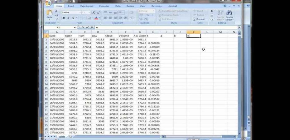
Before you begin, ensure your data is organized in an Excel spreadsheet. Whether it’s a list of measurements, voltage readings, or any other dataset, make sure it’s properly formatted and arranged.

Step 2: Square Each Value

Next, you’ll need to square each individual value in your dataset. This can be easily accomplished using Excel’s built-in functions. Simply create a new column and use the formula “=A1^2” (assuming your data is in column A) and drag it down to apply to all values.

Step 3: Find the Mean

Once you have the squared values, calculate the mean by using Excel’s average function. Select the range of squared values and apply the formula “=AVERAGE(A1:A10)” (adjusting the range as necessary).

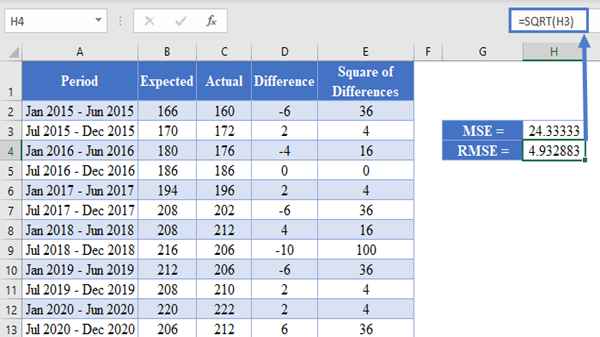
Step 4: Take the Square Root

Now comes the final step. Take the square root of the mean calculated in the previous step. Use Excel’s square root function by applying “=SQRT(A1)” (assuming the mean is in cell A1).

Congratulations! You’ve successfully calculated the RMS in Excel. This single value represents the root mean square of your dataset, providing valuable insights into its overall magnitude.

Advantages of Using Excel for RMS Calculations

Why bother with Excel for RMS calculations when there are specialized software and tools available? Here are some compelling reasons:

Accessibility

Excel is ubiquitous, readily available to most users. You don’t need to install additional software or learn complex interfaces. With a basic understanding of Excel functions, you can perform RMS calculations anytime, anywhere.

Flexibility

Excel offers unparalleled flexibility, allowing you to customize formulas, analyze data visually, and integrate with other tools seamlessly. Whether you’re dealing with small datasets or massive spreadsheets, Excel can handle it all.

Cost-Effectiveness

Compared to specialized software, Excel is cost-effective. There’s no need to invest in expensive licenses or subscriptions. With Excel, you’re leveraging a powerful tool at no additional cost.

Conclusion

In conclusion, mastering the art of calculating RMS in Excel opens up a world of possibilities. Whether you’re analyzing electrical signals, processing financial data, or conducting scientific experiments, the RMS value provides invaluable insights. By following the simple steps outlined in this guide, you can harness the power of Excel to compute RMS with ease. So why wait? Start crunching numbers and unlocking insights today!

Read Also

• Überzetsen: Mastering the Art of Language Translation for Multilingual Marketing Excellence
• Férarie: A Tale of Automotive Excellence and Italian Engineering Mastery
• 5 Easy Ways to Freeze Row and Column in Microsoft Excel
• 5 Ways to Deliver Excellent and Consistent Customer Service
• Bogo – Meta Shuts Down Fan Favorite VR Game
• How to Make a Yard Sale Listing on Craigslist